The Engineering Handbook for GRPO + LoRA with Verl: Training Qwen2.5 on Multi-GPU

Community Article Published January 2, 2026

The release of DeepSeek-R1 marked a paradigm shift in post-training, effectively showcasing the power of Reinforcement Learning with Verifiable Rewards (RLVR). Building on principles solidified in research like Tulu 3, R1 proved that Group Relative Policy Optimization (GRPO) could induce advanced reasoning capabilities by eliminating the memory-heavy value function, significantly reducing the compute overhead compared to traditional PPO.

However, moving from theory to execution requires robust distributed orchestration. While tools like Unsloth are excellent for memory-efficient training, verl provides the sophisticated distributed framework required for industrial production environments. As a primary tool for teams at ByteDance and other top labs, it is widely used in industry for high-throughput RL.

Yet, the power of an enterprise-grade framework often comes with a steep learning curve. Configuring Verl for high-performance workloads in cloud environments remains a non-trivial task, often requiring developers to move beyond the base documentation to resolve subtle system-level constraints and stability issues that emerge during distributed training.

This handbook documents the exact engineering path to setting up a stable, high-performance Multi-GPU GRPO + LoRa pipeline for the Qwen2.5–3B-Instruct model. We will address the common setup hurdles, resolve hidden environment conflicts, and optimize a training loop that converges in hours rather than days.

The Stack: Why We Chose This Architecture

Before we touch the terminal, we need to define our constraints. We are optimizing for efficiency and stability.

1. The Algorithm: GRPO (Group Relative Policy Optimization)

Traditional PPO (Proximal Policy Optimization) typically relies on four components loaded into VRAM: an Actor, a Critic (Value Function), a Reference, and a Reward model. The Critic is often the main bottleneck: it is usually comparable in size to the Actor, effectively doubling memory usage and increasing training overhead.

GRPO optimizes this by changing how the baseline is estimated.

Instead of training a separate Value Function (Critic) to predict expected returns, GRPO samples a group of responses (e.g., G = 5) for the same prompt. Each response is scored, and the group’s average reward is used as the baseline. Individual responses are then reinforced or penalized based on how they perform relative to this group average.

In verifiable reasoning tasks (RLVR), this allows us to operate without a learned Critic model entirely, relying instead on the ground-truth reward function.

Wins:

~50% lower VRAM usage by eliminating the need for a generic Value Function model.
Faster and simpler training loops (no Critic loss to compute).
Self-Correction: Encourages the model to beat its own average, naturally promoting stronger reasoning.

2. The Model: Qwen 2.5 3B Instruct

We are using Qwen 2.5 3B Instruct as our base.

Why 3B? It is the efficiency “sweet spot.” It is small enough to iterate quickly (high throughput) but intelligent enough to actually learn GSM8K math reasoning.
Why Instruct? Starting from an instruct-tuned checkpoint provides a stable “Cold Start” for RL, preventing the gibberish output often seen when RL-tuning base models from scratch.

3. The Framework: VERL + vLLM

We use Verl for orchestration and vLLM for generation.

The Challenge: RL Post-Training is a hybrid workload. It alternates between Generation (memory bandwidth bound) and Training (compute bound).
The Solution: Verl manages the complex state passing between the training loop and the inference engine (e.g. vLLM), allowing us to saturate our A100s.

Phase 1: The Infrastructure Setup

We are deploying this on a RunPod instance with 4x NVIDIA A100 (80GB) SXM GPUs.

Base Image: runpod/pytorch:1.0.2-cu1281-torch280-ubuntu2404
Goal: A clean, reproducible Conda environment.

Step 1: Initialize the Environment

First, we install a fresh Miniconda instance to decouple our environment from the system Python. This ensures a clean slate and prevents version conflicts with pre-installed packages.

# 1. Install Miniconda (if not present)  
wget https://repo.anaconda.com/miniconda/Miniconda3-latest-Linux-x86_64.sh  
bash ./Miniconda3-latest-Linux-x86_64.sh

Next, we initialize the Python environment. We are utilizing Python 3.12 (as also instated on the official verl installation page) to ensure full compatibility with the latest framework.

# 2. Create the environment  
conda create -n verl python=3.12 -y  
conda activate verl

Finally, we clone the framework repository and enter the working directory.

# 3. Clone the repository  
git clone https://github.com/volcengine/verl  
cd verl

Step 2: Installation and Framework Setup

Verl provides a convenience script (install_vllm_sglang_mcore.sh) to handle the complex dependency tree. This script automates the installation of heavy-duty infrastructure like vLLM, SGLang, and Megatron-LM.

First, run the script to install the base dependencies:

# 1. Run the official script for base dependencies  
chmod +x ./scripts/install_vllm_sglang_mcore.sh  
bash ./scripts/install_vllm_sglang_mcore.sh

Note: It is normal for this to hang on “Building Megatron-LM” for 15+ minutes.

Once the base infrastructure is ready, finalize the Verl installation by installing it in editable mode:

# 3. Install Verl  
pip install --no-deps -e .

💡 Pro Note: If you are working with specific previous commit hashes of Verl or find yourself in an environment where Python 3.12 triggers recursion or import errors you can’t solve, the most stable fallback is to switch to Python 3.11. If you do this, the automated script may fail to find a matching Flash Attention binary. In that case, you must manually install the pre-compiled wheel for your specific system (Python 3.11, CUDA 12.x) from the Flash Attention Releases page to ensure the installation works correctly.

Phase 2: The Data Pipeline

Reinforcement learning is sensitive to data formatting. A common pitfall is feeding raw datasets into the trainer without aligning the prompt structure with the reward function.

For this replication, we use the standard GSM8K dataset. Verl provides a pre-processing script, but we need to run it explicitly to generate the parquet files that the trainer expects.

Format the Dataset

Run the pre-processor to structure the GSM8K train/test splits.

# This generates 'train.parquet' and 'test.parquet' in ./data/gsm8k  
python3 examples/data_preprocess/gsm8k.py --local_dir "./data/gsm8k"

Note on “Think Tags”: Unlike DeepSeek-R1, the standard Verl pre-processor uses a generic Chain-of-Thought prompt (“Let’s think step by step”). It does not inject <think> tags by default. This means our model will learn to reason in plain text, which is mathematically equivalent but requires different parsing logic during evaluation.

Phase 3: The Training

With the environment fixed and data prepped, we move to the core training logic. We will use the LoRA + GRPO workflow.

Verl provides a reference script for this: examples/grpo_trainer/run_qwen2_5-3b_gsm8k_grpo_lora.sh.

Let’s look at the default configuration. While this script contains the correct algorithmic skeleton, the default hyperparameters (shown below) are extremely conservative. We will change them based on our needs and environment.

set -x  
  
python3 -m verl.trainer.main_ppo \  
    algorithm.adv_estimator=grpo \  
    trainer.val_before_train=False \  
    data.train_files=$HOME/data/gsm8k/train.parquet \ # YOU MAY NEED TO CHANGE THIS  
    data.val_files=$HOME/data/gsm8k/test.parquet \ # YOU MAY NEED TO CHANGE THIS  
    data.train_batch_size=16 \  
    data.max_prompt_length=512 \  
    data.max_response_length=1024 \  
    data.filter_overlong_prompts=True \  
    data.truncation='error' \  
    data.shuffle=False \  
    actor_rollout_ref.model.path=Qwen/Qwen2.5-3B-Instruct \  
    actor_rollout_ref.model.lora_rank=64 \  
    actor_rollout_ref.model.lora_alpha=32 \  
    actor_rollout_ref.actor.optim.lr=3e-6 \  
    actor_rollout_ref.model.use_remove_padding=True \  
    actor_rollout_ref.actor.ppo_mini_batch_size=16 \  
    actor_rollout_ref.actor.ppo_micro_batch_size_per_gpu=40 \  
    actor_rollout_ref.actor.use_kl_loss=True \  
    actor_rollout_ref.actor.kl_loss_coef=0.001 \  
    actor_rollout_ref.actor.kl_loss_type=low_var_kl \  
    actor_rollout_ref.actor.entropy_coeff=0 \  
    actor_rollout_ref.model.enable_gradient_checkpointing=True \  
    actor_rollout_ref.actor.fsdp_config.param_offload=False \  
    actor_rollout_ref.actor.fsdp_config.optimizer_offload=False \  
    actor_rollout_ref.rollout.log_prob_micro_batch_size_per_gpu=40 \  
    actor_rollout_ref.rollout.tensor_model_parallel_size=2 \  
    actor_rollout_ref.rollout.name=vllm \  
    actor_rollout_ref.rollout.gpu_memory_utilization=0.6 \  
    actor_rollout_ref.rollout.n=5 \  
    actor_rollout_ref.rollout.load_format=safetensors \  
    actor_rollout_ref.rollout.layered_summon=True \  
    actor_rollout_ref.ref.log_prob_micro_batch_size_per_gpu=40 \  
    actor_rollout_ref.ref.fsdp_config.param_offload=True \  
    algorithm.use_kl_in_reward=False \  
    trainer.critic_warmup=0 \  
    trainer.logger='["console","wandb"]' \  
    trainer.project_name='verl_grpo_example_gsm8k' \  
    trainer.experiment_name='qwen2.5_3b_grpo_lora' \  
    trainer.n_gpus_per_node=2 \ # CHANGE THIS TO 4  
    trainer.nnodes=1 \  
    trainer.save_freq=20 \  
    trainer.test_freq=5 \  
    trainer.total_epochs=15 $@  
  
    # actor_rollout_ref.actor.ppo_mini_batch_size=256 \  
    # data.train_batch_size=1024 \  
    # trainer.n_gpus_per_node=8 \  
    # actor_rollout_ref.model.use_shm=True \

1. Critical Hyperparameter Focus

Before running the default script, we must identify the bottlenecks. The default values provided in the example are extremely inefficient for a 4xA100 80GB.

trainer.n_gpus_per_node (Default: 2): The default script assumes a 2-GPU setup. We must increase this to 4 to fully utilize our specific hardware node.
data.train_batch_size (Default: 16): This is the Global Batch Size (total experiences gathered per training step). A default of 16 is relatively low for this scale of training. We will increase this significantly (to 1024) to potentially improve the stability of the policy updates and overall throughput.
ppo_micro_batch_size_per_gpu (Default: 40): This determines how many samples are processed on the GPU in a single pass. On high-end hardware like the A100, increasing this value is usually necessary to better utilize the available compute capacity.
ppo_mini_batch_size (Default: 16): This controls the batch size used specifically during the PPO update loop. The default is quite small, which can lead to inefficient processing on large GPUs. We will scale this up (to 512) to process the collected data in larger, more efficient chunks.
rollout.tensor_model_parallel_size This controls how the model is distributed across GPUs. The default often assumes model parallelism (sharding) is required. For a smaller model like Qwen 2.5 3B, sharding may introduce unnecessary communication overhead, so we will investigate if Data Parallelism is a better fit.
rollout.gpu_memory_utilization (Default: 0.6): This parameter limits how much VRAM vLLM can reserve for the KV cache. On 80GB cards, leaving this at 0.6 leaves a significant amount of memory unused, which we can likely reclaim for performance.
rollout.n (Default: 5): This is the number of outputs generated per prompt to estimate the group baseline. We will experiment with this value to find the right balance between a stable baseline estimator and speed.

Finally, we will retain the default values for the model training hyperparameters, including trainer.total_epochs (15), optim.lr (3e-6), and the LoRA configuration (rank=64, alpha=32). While experimenting with these values is critical for maximizing final model performance, this post centers on the engineering challenges of the GRPO loop itself rather than the hyperparameter search space.

2. Pre-Flight Checks (Don’t Burn Money and Time)

Once we edit the script parameters (which we will detail in the optimization section), there are two operational steps you should take before launching the run.

⚠️ The “WandB Login” Trap: The training script performs heavy initialization (loading the model to VRAM, compiling kernels) before it initializes the logger. If you haven’t authenticated WandB, the script will run for 5 minutes and then crash, wasting paid GPU time.

# Run this ONCE before training  
wandb login

The Monitoring Tool: To actually see if our optimizations work, we need real-time telemetry. nvitop is a great tool for this.

pip3 install nvitop  
nvitop

3. Launching the Baseline Experiment

Before executing the script, we modify the following hyperparameters to establish a high-throughput baseline. For this initial run, we will keep the model sharded across all GPUs (TP=4) but increase the batch sizes to properly load the A100s.

Open ./examples/grpo_trainer/run_qwen2_5-3b_gsm8k_grpo_lora.sh and update:

data.train_batch_size=1024
actor_rollout_ref.actor.ppo_mini_batch_size=512
actor_rollout_ref.rollout.tensor_model_parallel_size=4 (Matching our GPU count)

With the configuration set, grant execution permissions and launch the training loop:

chmod +x ./examples/grpo_trainer/run_qwen2_5-3b_gsm8k_grpo_lora.sh # ONCE  
./examples/grpo_trainer/run_qwen2_5-3b_gsm8k_grpo_lora.sh

This initiates the training with our “Baseline” configuration. From here, we will monitor everything to identify bottlenecks and iteratively optimize the setup.

Note: We start our experiment with parameters that differ significantly from the reference script, as using the original values would result in an estimated time to completion of several days.

4: Optimization and Finding The “Right” Things

Let’s analyze our first experiment run. The training has stabilized, and the ETA is hovering around 9.5 hours. This is functional, but the telemetry reveals we are leaving performance on the table.

Let’s look at the telemetry from the first 20 minutes:

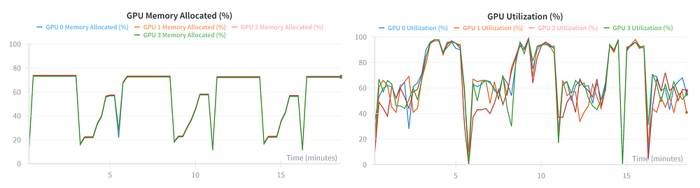
The Diagnosis:

VRAM (Left): This is the smoking gun. We are peaking at only ~75% usage. This means on every single A100, we are leaving ≈20GB of VRAM completely empty.
Utilization (Right): While the GPUs do spike to 100%, the graph is “noisy.” The lines for the four GPUs are jittery and don’t always overlap perfectly.
The Issue: This “jitter” usually indicates Communication Overhead. Because we set TP=4, the GPUs have to stop and synchronize gradients constantly.

The Root Cause: Oversharding

We configured tensor_model_parallel_size=4, which shards the model weights across all four GPUs. However, a 3B parameter model is tiny (approx. 6GB). By splitting such a small model four ways, we force the GPUs to spend precious time waiting for communication rather than just crunching numbers.

We are paying a “communication tax” for a model that doesn’t need it. We need to fix this.

Optimization 1: Switching to Data Parallelism (`TP=1`)

Our first move is to eliminate the communication overhead. We changed tensor_model_parallel_size from 4 to 1.

The Logic: A 3B parameter model is tiny. Sharding it across 4 GPUs (TP=4) forces the cards to constantly stop and exchange data. By switching to TP=1, we switch to Data Parallelism so each GPU runs its own independent replica of the model and just syncs gradients at the end.

The Result:

New ETA: ~6.5 Hours (-33% Training Time ✅)
The Impact: We instantly shaved off 3 hours just by removing the network bottleneck.

You might think: “Since we are putting the full model on each GPU instead of 1/4th of it, shouldn’t VRAM usage spike and solve our VRAM usage problem?”

Answer: No, the model is only ~6GB. Whether you store ~1.5GB (TP=4) or ~6GB (TP=1) on an 80GB A100, it’s a drop in the bucket.

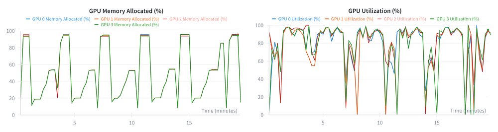
Let’s look at the new graph for this run:

Why this graph is “Prettier” (and Better):

Synchronization: Look at the colored lines (Blue, Orange, Red, Green). In the previous run, they were jittery and split apart. Here, they are glued together. This proves the GPUs are more synchronized, crunching numbers in parallel without waiting for each other.
The Remaining Problem: Notice that VRAM usage (Left) is still stuck at ~78%. We solved the latency issue (speeding up the run), but we haven’t solved the throughput issue (filling the memory). We are still starving the cards.

Test 1: Increasing Rollout Fidelity (`N=5` → `N=10`)

Before we attack the VRAM issue, we ran one algorithmic experiment.

In GRPO, the “Baseline” is calculated as the average reward of the group of outputs. Theoretically, increasing the number of rollouts (rollout.n) from 5 to 10 should reduce the variance of this estimator and lead to more stable training updates.

The Experiment: We changed actor_rollout_ref.rollout.n from 5 to 10 and launched the run. (Note: n=16 is the default value adopted in most papers, but we opted to test a smaller increment first to check the compute penalty).

The Result:

ETA: Jumped from 6.5 Hours to 11 Hours (+70% Training Time).
The Bottleneck: On-Policy RL is generation-bound. Because vLLM generates these sequences sequentially (or in batches that hit the decoding bottleneck), doubling the rollout count almost linearly increases the generation phase duration.

The Verdict: Negative ROI. While n=10 (or the academic standard n=16) might offer better convergence stability, the 70% cost increase is not justifiable for this specific workload. While complex tasks often require high rollout counts to effectively hill-climb, our 3B model is already converging well on GSM8K, so we are essentially spending 5 extra hours just to reduce a bit of noise.

Decision: Fallback to **N=5** for the final run.

Optimization 2: Solving VRAM Starvation (`rollout.gpu_memory_utilization`)

Now we attack the final inefficiency. Despite fixing the synchronization issues with TP=1, our VRAM usage was still plateauing at ~78%. This means we were failing to utilize the massive memory bandwidth of the A100s, which is critical for the generation phase.

The control lever for this is rollout.gpu_memory_utilization.

How it works: This parameter sets a hard ceiling on the memory budget allocated to the inference engine. It essentially controls how aggressively the system attempts to utilize available VRAM during the rollout phase.
The Constraint: This is a balancing act. If you set this value too high, the inference engine may consume so much memory that there is no room left for the training computations (gradients, optimizer states), causing an OOM crash. If you set it too low, you simply leave performance on the table.

The Experiment: Values of 0.9 (OOM Crash) and 0.7 (Still Underutilized) are tested as well.

The “Sweet Spot” for this 3B model on an 80GB card proved to be 0.8.

The Result:

ETA: Dropped from 6.5 hours to 6 Hours (-8% Training Time).
Total Speedup: Combined with Optimization 1, we have reduced training time by ~38% (9.5h to 6h).

Analyzing the Telemetry:

Let’s look at the final VRAM and Utilization graphs:

The Verdict: Saturation.

VRAM (Left): Usage now peaks at >95%. We are filling the cards to the brim.
Utilization (Right): The graph shows the healthy “Sawtooth” pattern we expect. Deep valleys during generation (where we unload optimizer states) and solid 100% peaks during training.

We have successfully tuned the system. The loop is stable, fast, and fully utilizes the hardware. We are ready to let it run.

⚡ War Story: The Step 80 Crash (Disk Full)

Just as we thought we were in the clear, the run crashed at Step 80/105.

The Cause: Disk Full. I had underestimated the sheer size of the checkpoints. My container's root volume filled up quickly after several checkpoints, killing the last checkpoint saving process mid-write.

The Fix: If this happens to you, do not restart from scratch. Verl has a built-in resume capability, but you need to clean up the mess first.

Delete the Corruption: The crash happened during the save, leaving a half-written checkpoint folder. You should delete this manually, or the resume logic may choke on it.

# Example: Deleting the corrupted step 80 folder  
rm -rf /workspace/verl/checkpoints/verl_grpo_example_gsm8k/qwen2.5_3b_grpo_lora/global_step_80

2. Free Up Disk Space: You must reclaim space before the next save. Start by deleting any non-essential files in your setup, such as unused datasets or checkpoints from previous experiments. If you don’t have these files, the most effective method is removing older, intermediate checkpoints from the current run.

❗ Consider uploading these checkpoints to platforms like Hugging Face before you proceed!

# Example: Deleting 3 checkpoint folders to open up disk space  
rm -rf /workspace/verl/checkpoints/verl_grpo_example_gsm8k/qwen2.5_3b_grpo_lora/global_step_20  
rm -rf /workspace/verl/checkpoints/verl_grpo_example_gsm8k/qwen2.5_3b_grpo_lora/global_step_40  
rm -rf /workspace/verl/checkpoints/verl_grpo_example_gsm8k/qwen2.5_3b_grpo_lora/global_step_60

Enable Auto-Resume: Open your running script (run_qwen2_5-3b_gsm8k_grpo_lora.sh) and add this flag to the end of the python command:

trainer.resume_mode="auto" \

4. Relaunch: Run the script again.

./examples/grpo_trainer/run_qwen2_5-3b_gsm8k_grpo_lora.sh

Prevention: To avoid this manual cleanup in future runs, you can configure the trainer to manage storage automatically. Adding trainer.save_total_limit=3 will force the system to keep only the three most recent checkpoints, automatically deleting the oldest ones as it goes. You should also consider increasing trainer.save_freq (e.g., from 20 to 50) to write to disk less frequently, reducing the cumulative pressure on your storage volume.

5: Mission Accomplished

After resolving the disk space crash, the trainer automatically detected the last valid state (Step 60), loaded the heavy optimizer states, and resumed seamlessly. We successfully reached Step 105.

The Outcome: The script completed the full 15 epochs. While we lost some wall-clock time due to the crash, we experienced zero data loss.

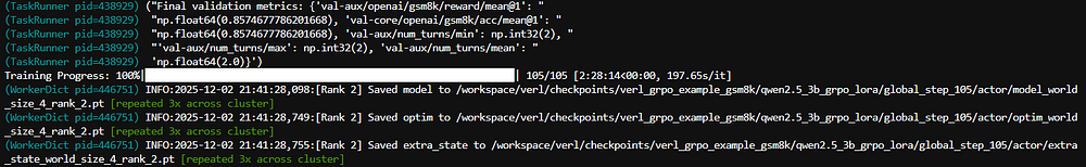
Note: You might see a long “Signal Killed” or “Process Terminated” error in the terminal at the very end. Don’t panic. This is usually just the WandB background process getting killed before it closes gracefully. As long as your final checkpoint exists in the folder, you are safe.

1. System Health: The “Heartbeat”

Let’s look at the full run’s telemetry (Run 1 + Run 2 stitched together).

Analysis: This graph validates our optimizations.

VRAM (Left): The usage peaks consistently touch ~95% without triggering OOM errors. We are utilizing nearly every gigabyte of the A100s.
Utilization (Right): The pattern is stable. We see dense blocks of 100% utilization (Training Phase) interspersed with the lower-utilization Generation Phase. There is no degradation in performance over time.

2. The Learning Curve: Reward Mean

Did the model actually align with our reward criteria? This is a critical graph that tracks our progress.

Analysis:

The Climb: The model started with a mean reward of ~0.55 and climbed steadily to ~0.90.
The Resume (Pink vs. Blue): Notice the transition from the Pink line (Run 1) to the Blue line (Run 2) at Step 60. The lines connect perfectly. This visually confirms that our resume operation was precise.

3. Policy Drift: The KL Divergence

We check if the model “collapsed” or drifted too far.

Analysis:

The KL loss rises monotonically (steadily) but remains bounded, peaking around 0.0027. This indicates a healthy drift.

If the KL loss stayed flat (around 0.0), the model would not be learning anything new.
If the KL loss spiked vertically (e.g., greater than 0.1), the model would likely be outputting gibberish.

Result:

The model explored new strategies while staying close enough to the reference distribution to maintain coherent language.

4. The Stability Check: Gradient Norm

We check the gradient norm to ensure the model updates were numerically stable and didn’t suffer from “exploding gradients”: a common issue in RL that leads to model collapse.

Analysis:

No Spikes: The graph is smooth with no massive vertical jumps. In unstable runs, you would see this line shoot up vertically indicating that the model weights are being destroyed.
Healthy Convergence: We see a sharp, healthy decline in the first 20 steps (dropping from ~0.024 to ~0.007) as the model adapted to the new reward structure.
The Plateau: From Step 40 onwards, the norm stabilizes around 0.005. This confirms that our learning rate was correct and the optimization landscape was smooth.

Result: The training remained numerically stable throughout the entire run. The gradients were consistently bounded, and the “resume” operation (where the blue line takes over) introduced no instability or spikes.

5. Response Length: The Preference for Brevity

Finally, we arrive at the most fascinating metric of this entire run.

In recent “Reasoning Model” breakthroughs (like DeepSeek-R1), the hallmark behavior is Extended Thinking. As the model gets smarter, it generates more tokens, exploring different paths before answering. We expected our graph to drift upward.

It did the exact opposite.

The Observation: Our mean response length started at ~290 tokens and monotonically decreased to ~220 tokens. The model didn’t just get smarter (0.55 -> 0.90 Reward); it got faster.

The Investigation: Why did our model choose brevity over depth? To understand this, we have to look at the source code. The incentive structure defines the behavior.

Let’s inspect how verl calculates rewards for GSM8K. I dug into the source code at verl/utils/reward_score/gsm8k.py:

def compute_score(solution_str, ground_truth, method="strict", format_score=0.0, score=1.0):  
    answer = extract_solution(solution_str=solution_str, method=method)  
    if answer is None:  
        return 0  
    else:  
        if answer == ground_truth:  
            return score  # Returns 1.0  
        else:  
            return format_score # Returns 0.0

The Smoking Gun: The reward function is Binary and Outcome-Based.

Correct Answer: +1.0 Reward.
Detailed Reasoning: +0.0 Bonus.
Wrong Answer: 0.0 Reward.

Simultaneously, the GRPO algorithm includes a KL Divergence Penalty. The model is penalized for every token that deviates from the reference model.

The Equation: Total Reward = (Binary Score) - (KL Penalty * Length)
The Strategy: Since “thinking longer” gives zero additional reward but incurs more KL penalty (and increases the chance of a hallucination), the model converged on the most efficient path: “Shut up and calculate.”

The Contrast (Open-R1): Compare this to the reward functions used in projects like Hugging Face’s Open-R1. In their rewards.py, they often experiment with specific bonuses for formatting or reasoning steps (using XML tags like <think>).

Open-R1: Incentivizes the process of thinking.
Our Config: Incentivizes the result of thinking.

The Verdict: We didn’t train a philosopher; we trained a ruthless efficiency expert. Because GSM8K is relatively “easy” for Qwen 2.5 3B Instruct based model, it realized that verbose reasoning was just expensive fluff. It optimized to find the correct answer in the fewest tokens possible to maximize its reward-to-penalty ratio.

Phase 6: Validation & The “Benchmark Trap”

Now that training is complete, we need to answer the ultimate question: Did we actually make the model better?

1. Internal Validation: The “Overkill” Realization

First, let’s look at the validation accuracy on the held-out test set during training. This measures how well the model performs on the specific prompt format we trained on.

The Good News:

Massive Jump: Validation accuracy rocketed from ~59% (Step 0) to ~85% (Step 100). This confirms the GRPO algorithm works. The model successfully aligned itself with the reward function.

The “Brutal” Truth:

We Wasted Time: Look at the curve. The model reached ~83% accuracy within the first 3 Epochs. The remaining 12 epochs spent hours of GPU time fighting for a marginal +2% gain.
Lesson Learned: For small models (3B) using LoRA with hyperparameters similar to what we used, convergence happens fast. In future runs, we can safely cut the trainer.total_epochs from 15 down to 5, saving ~60% of our compute budget without sacrificing meaningful performance.

2. External Evaluation: The “Format” Reality Check

The internal graph looks great, but does it transfer to standardized benchmarks? We ran both the base model (Qwen 2.5 3B Instruct) and our finetuned model through LM Evaluation Harness to get an unbiased score.

# We ran standard GSM8K and GSM8K-CoT tasks  
lm_eval \  
    --model vllm \  
    --model_args pretrained={MODEL},tensor_parallel_size={X},gpu_memory_utilization=0.8,data_parallel_size={Y} \  
    --tasks gsm8k,gsm8k_cot \  
    --batch_size auto \  
    --output_path ./results

The Results:

Analysis: Why didn’t we see the +25% jump here?

This reveals a critical nuance in RL:

Format Overfitting: Our internal validation score (85%) comes from the specific prompt template used in the training loop. The model became a “Specialist” in solving problems when asked in that specific way.
Benchmark Mismatch: LM Eval Harness uses standardized few-shot prompts that differ from our training environment.
The “Strict” Win: Notice that we saw the biggest gains in Strict Match (+3.7% and +2.9%). This makes perfect sense. Our reward function was binary (1.0 for exact match, 0.0 otherwise). We effectively trained the model to be more pedantic and precise with its final answer formatting, which helps strictly-graded metrics but doesn’t necessarily radically improve the “Flexible” reasoning score (which the Base model was already good at).

Conclusion: We successfully specialized the model to our target format and improved its strict adherence to answer requirements, but we did not fundamentally transform its reasoning capabilities on out-of-distribution prompts. This is a classic trade-off in Policy Optimization.

The Road Ahead

With this experiment, we have achieved something critical: We established a stable, high-throughput GRPO infrastructure on A100s.

Most RL projects fail not because the math is wrong, but because the engineering is unstable. OOM crashes, inefficient batching, or silent data corruption kill more projects than bad algorithms do. By solving the system constraints like VRAM saturation, TP strategies, and resume logic, we have built a solid foundation.

Now that the engine is running perfectly, future work can focus on tuning the system. Here are the most high-leverage areas to explore next:

1. Reward Engineering: From Efficiency to Reasoning

Our analysis revealed a fascinating insight. A binary reward system plus a KL penalty drives the model toward Maximum Efficiency (shorter answers) in scenarios like ours. To replicate the “Deep Reasoning” behaviors seen in models like R1 where the model “thinks” for thousands of tokens, we cannot simply rely on outcome-based scoring. A natural next step would be investigating Process-Based Rewards (P-RMs) or regex-guided format rewards that specifically incentivize the act of thinking, rather than just the final answer.

2. Breaking the Format Trap (Dataset Strategy)

We trained on GSM8K using a specific template, which made the model a specialist in that domain. To build a truly robust reasoning model, the data pipeline needs to evolve. Future iterations could explore Data Diversity by mixing in other datasets. More importantly, we should look at Template Randomization. Varying the prompt structure during the rollout phase would likely prevent the model from overfitting to a specific syntax and force it to generalize the underlying logic.

3. Fine-Grained Hyperparameter Tuning

In this run, we intentionally fixed the model architecture hyperparameters (LoRArank 64, alpha 32, epochs 15) to standard defaults. This was a deliberate choice to isolate the system stability variables. With the pipeline now stable, one could aggressively optimize these values. For instance, experimenting with significantly shorter training schedules (Early Stopping at Epoch 5) or dynamic learning rate schedulers could yield the same performance with a fraction of the compute budget.

We have cleared the path. The hardware is saturated, the loop is closed, and the baseline is set. Building a stable RL infrastructure is often the hardest problem to solve, and that is exactly what we delivered here.

Conclusion

This project highlights that efficient RL training is not solely about algorithmic choices, but also about engineering the underlying pipeline. By optimizing the training infrastructure and memory configurations, the total training duration was significantly reduced without compromising model convergence. With the final configuration, the total cost is approximately $40, based on pricing calculated from RunPod’s Secure Pod offering.

The final model weights from this run are available on Hugging Face:

🤗 Hugging Face: Weyaxi/Qwen2.5–3B-Instruct-GRPO-GSM8K-LoRa-verl

A Note on Reproducibility & Feedback

Deep Reinforcement Learning is notoriously sensitive to hardware, seed, and hyperparameter variations. The results and graphs presented here reflect our specific experimental conditions on A100 GPUs. While I have strived for rigorous accuracy in interpreting the telemetry, the “art” of RL often invites multiple interpretations.

If you notice a discrepancy, have a different interpretation of the data, or spot an error in the stack, please reach out. This is a living document, and I welcome the opportunity to correct or refine the findings based on community feedback.

Acknowledgements

I would like to extend a special thank you to Maxime Labonne (Liquid AI) for his detailed feedback and technical insights on this article. His expertise was instrumental in refining the depth and accuracy of this post.

References

DeepSeek-R1: Incentivizing Reasoning Capability in LLMs via Reinforcement Learning https://arxiv.org/abs/2501.12948
Proximal Policy Optimization Algorithms (PPO) https://arxiv.org/abs/1707.06347
DeepSeekMath: Pushing the Limits of Mathematical Reasoning in Open Language Models https://arxiv.org/abs/2402.03300
Qwen2.5 Technical Report https://arxiv.org/abs/2412.15115
Tulu 3: Pushing Frontiers in Open Language Model Post-Training https://arxiv.org/abs/2411.15124
Verl Performance Tuning Guide https://verl.readthedocs.io/en/latest/perf/perf_tuning.html
Verl RL(HF) algorithms with LoRA Support https://verl.readthedocs.io/en/latest/advance/ppo_lora.html
Verl Group Relative Policy Optimization (GRPO) https://verl.readthedocs.io/en/latest/algo/grpo.html
Unsloth: Reinforcement Learning (RL) Guide https://docs.unsloth.ai/get-started/reinforcement-learning-rl-guide
Github: Open-R1 (Hugging Face) https://github.com/huggingface/open-r1
GitHub: Verl (Volcengine) https://github.com/volcengine/verl
GitHub: vLLM https://github.com/vllm-project/vllm
GitHub: nvitop https://github.com/XuehaiPan/nvitop
Dataset: GSM8K (OpenAI) https://huggingface.co/datasets/openai/gsm8k
GitHub: LM Evaluation Harness https://github.com/EleutherAI/lm-evaluation-harness
GitHub: Flash Attention Releases https://github.com/Dao-AILab/flash-attention/releases
Miniconda Installation Guide https://www.anaconda.com/docs/getting-started/miniconda/install#linux-terminal-installer
Runpod GPU Cloud Pricing https://www.runpod.io/pricing

Community

Upload images, audio, and videos by dragging in the text input, pasting, or clicking here.

Tap or paste here to upload images

· Sign up or log in to comment

Upvote

The Engineering Handbook for GRPO + LoRA with Verl: Training Qwen2.5 on Multi-GPU

The Stack: Why We Chose This Architecture

1. The Algorithm: GRPO (Group Relative Policy Optimization)

2. The Model: Qwen 2.5 3B Instruct

3. The Framework: VERL + vLLM

Phase 1: The Infrastructure Setup

Step 1: Initialize the Environment

Step 2: Installation and Framework Setup

Phase 2: The Data Pipeline

Format the Dataset

Phase 3: The Training

1. Critical Hyperparameter Focus

2. Pre-Flight Checks (Don’t Burn Money and Time)

3. Launching the Baseline Experiment

4: Optimization and Finding The “Right” Things

Optimization 1: Switching to Data Parallelism (TP=1)

Test 1: Increasing Rollout Fidelity (N=5 → N=10)

Optimization 2: Solving VRAM Starvation (rollout.gpu_memory_utilization)

⚡ War Story: The Step 80 Crash (Disk Full)

5: Mission Accomplished

1. System Health: The “Heartbeat”

2. The Learning Curve: Reward Mean

3. Policy Drift: The KL Divergence

4. The Stability Check: Gradient Norm

5. Response Length: The Preference for Brevity

Phase 6: Validation & The “Benchmark Trap”

1. Internal Validation: The “Overkill” Realization

2. External Evaluation: The “Format” Reality Check

The Road Ahead

1. Reward Engineering: From Efficiency to Reasoning

2. Breaking the Format Trap (Dataset Strategy)

3. Fine-Grained Hyperparameter Tuning

Conclusion

A Note on Reproducibility & Feedback

Acknowledgements

References

Community

Optimization 1: Switching to Data Parallelism (`TP=1`)

Test 1: Increasing Rollout Fidelity (`N=5` → `N=10`)

Optimization 2: Solving VRAM Starvation (`rollout.gpu_memory_utilization`)